Programming Grover’s algorithm and Deutsch–Jozsa algorithm

In my previous blog on Grover’s algorithm and Deutsch–Jozsa algorithm, I promised to post a blog on how to program them. Now its time to full fill the promise.

Please, if you don’t familiar with how these algorithms works, please go through the above two blogs first.

Deutsch–Jozsa algorithm

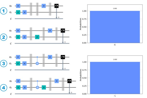
First, lets program the single quantum bit scenario. Here we can think of 4 types of oracle functions.

1. f(x) = 0
2. f(x) = 1
3. f(x) = x
4. f(x) = 1 – x

As we can see the first two functions are constant and the remaining two functions are balanced. Let’s write a program to see these oracles in action.

	from matplotlib import pyplot as plt
	import numpy as np
	from qiskit import *
	from qiskit.tools.visualization import plot_histogram
	# Creating a circuit with 3 quantum bits and 2 classical bit
	qc = QuantumCircuit(2,1)
	# Preparing inputs
	qc.h(0)
	qc.x(1)
	qc.h(1)
	qc.barrier()
	# Oracle function 1
	# Oracle function 2
	#qc.x(1)
	# Oracle function 3
	#qc.cx(0,1)
	# Oracle function 4
	#qc.cx(0,1)
	#qc.x(1)
	qc.barrier()
	# Preparing output
	qc.h(0)
	qc.barrier()
	# measuring the results
	qc.measure(0,0)
	qc.draw(output='mpl')
	# Running the experiment in simulator
	simulator = Aer.get_backend('qasm_simulator')
	result = execute(qc,backend=simulator,shots=1024).result()
	plot_histogram(result.get_counts())

view raw

Deutsch–Jozsa_one_bit.py

hosted with ❤ by GitHub

We know that after applying the oracle y becomes -> y XOR f(x).

In the case of f(x) = 0, y XOR f(x) = y. This is why we are not doing anything for function 1 in line no 17. In the case of f(x) = 1, y XOR f(x) = y’. This is why we add a not gate to Y in line 19.

Likewise, please try to understand what we are doing in functions 3 and 4 to achieve y XOR f(x)

By un-commenting the respective lines for each function we can take the following 4 circuits and results.

 

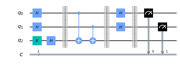
Now, let’s do the same exercise for a multi-qubit scenario.

	from matplotlib import pyplot as plt
	import numpy as np
	from qiskit import *
	# Creating a circuit with 3 quantum bits and 2 classical bit
	qc = QuantumCircuit(3,2)
	# Preparing inputs
	qc.h(0)
	qc.h(1)
	qc.x(2)
	qc.h(2)
	qc.barrier()
	# Oracle function
	qc.cx(0,2)
	qc.cx(1,2)
	qc.barrier()
	# Preparing output
	qc.h(0)
	qc.h(1)
	qc.barrier()
	# measuring the results
	qc.measure(0,0)
	qc.measure(1,1)
	qc.draw(output='mpl')
	# Running the experiment in simulator
	simulator = Aer.get_backend('qasm_simulator')
	result = execute(qc,backend=simulator,shots=1024).result()
	plot_histogram(result.get_counts())
	# Running the experiment in actual IBM quantum computer
	IBMQ.load_account()
	job = execute(qc,IBMQ.get_provider('ibm-q').get_backend('ibmq_16_melbourne'))
	# Job status = queued -> finished
	job_monitor(job)
	plot_histogram(job.result().get_counts())

view raw

Deutsch–Jozsa.py

hosted with ❤ by GitHub

In line 32 we draw the circuit. Which will give an output as follows.

In line 37 and 46 we plot the results from the simulation and the real quantum computer outputs.

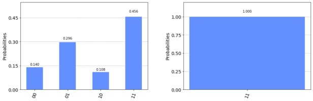
As we can see even though 11 has a high probability. Real quantum results are altered by the noise of quantum gates.

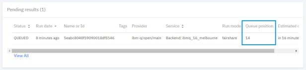
Here we are loading our IBM account details using IBMQ.load_account() command. If you haven’t configured your environment with IBM, you can create an account, copy the token from here and execute the command IBMQ.save_account(‘token’).

After submitting to IBM, our computation will be queued and it will take some time to complete. Meanwhile, we can view our queue position on our account home page.

For the constant functions, we do not need an oracle. Which means we can simply re-run the above algorithm again after commenting out the lines 17 and 18.

Grover’s algorithm

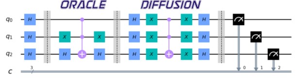
Before moving into the Grover’s algorithm we have prepare an oracle function. The functionality of the oracle should be to inverse the amplitude of the number we search when input with superposition of all states.

It turns out we can achieve this using the following simple circuit. This circuit will inverse the amplitude of 5 = 101

To visualize the effect of amplitude inverse, we have to use the statevector_simulator. As a side note, we cannot use measurement gates when we are using the statevector_simulator since the act of measuring collapse the qubits.

	from matplotlib import pyplot as plt
	import numpy as np
	from qiskit import *
	from qiskit.tools.visualization import plot_histogram
	from qiskit.tools.visualization import plot_state_city
	from qiskit.providers.aer import StatevectorSimulator
	# Creating quantum circuit with 3 qubits
	qc = QuantumCircuit(3)
	# Preparing inputs
	qc.h(0)
	qc.h(1)
	qc.h(2)
	qc.barrier()
	# Oracle function for number 5 = 101
	qc.x(1)
	qc.h(2)
	qc.ccx(0,1,2)
	qc.x(1)
	qc.h(2)
	qc.barrier()
	qc.draw(output='mpl')
	backend = Aer.get_backend('statevector_simulator')
	result = execute(qc, backend, shots=1024).result()
	# Get the statevector from result().
	statevector = result.get_statevector(qc)
	plot_state_city(statevector)

view raw

Oracle_for_number5.py

hosted with ❤ by GitHub

In line 33 we plot use the plot_state_city to represent the statevector as an amplitude graph which gives the following output.

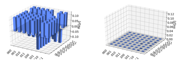
Here, we can see the amplitude is inversed for 101 which is number 5.

Next step is to add the diffusion operator to the same circuit. Which will invert and boost the amplitude of number 5.

	from matplotlib import pyplot as plt
	import numpy as np
	from qiskit import *
	from qiskit.tools.visualization import plot_histogram
	# Creating quantum circuit with 3 qubits and 3 classical bits
	qc = QuantumCircuit(3,3)
	# Preparing inputs
	qc.h(0)
	qc.h(1)
	qc.h(2)
	qc.barrier()
	# Oracle function for number 5 = 101
	qc.x(1)
	qc.h(2)
	qc.ccx(0,1,2)
	qc.x(1)
	qc.h(2)
	qc.barrier()
	# diffusion operator
	qc.h(0)
	qc.h(1)
	qc.h(2)
	qc.x(0)
	qc.x(1)
	qc.x(2)
	qc.ccx(0,1,2)
	qc.x(0)
	qc.x(1)
	qc.x(2)
	qc.h(0)
	qc.h(1)
	qc.h(2)
	qc.barrier()
	# measuring the output
	qc.measure(0,0)
	qc.measure(1,1)
	qc.measure(2,2)
	qc.draw(output='mpl')
	# Running the experiment in simulator
	simulator = Aer.get_backend('qasm_simulator')
	result = execute(qc,backend=simulator,shots=1024).result()
	plot_histogram(result.get_counts())

view raw

Grover_full.py

hosted with ❤ by GitHub

And we get the final result as follows.

Thank You 🙂